- Network Sites:
-
 EEPower Day is a free 1-day virtual conference. Learn More
In this page, we will expand and reinforce our understanding of power dissipation in AC circuits. As the title suggests, calculating AC power results in an expression that can be interpreted as two separate components: average power and sinusoidal power.
AC power is an expansive subject, but it’s very important to remember that it all starts with the fundamental definition of electrical power: current times voltage. In an AC circuit, though, we can’t represent current or voltage with a single number. Rather, the current and voltage change from one moment to the next, and consequently we use a mathematical expression (with the variable t, for time) instead of a number.
As you know, the expressions that we use to represent AC signals are sine or cosine functions characterized by an amplitude, a frequency, and a phase. In this page, we’ll use cosine:
Here, V and I represent the peak value of the sinusoids, and ω is the angular frequency present throughout the circuit.
The use of a negative sign with the phase term indicates that the waveform will be delayed by a phase of θV or θI relative to some other waveform. And actually, we can eliminate one of these phase terms by choosing the voltage signal as the reference waveform, because the reference waveform is assumed to have a phase of zero. The second phase term then becomes simply θ (rather than θI), and this θ represents the phase difference between voltage and current.

To generate a time-domain expression for power, we multiply V(t) and I(t):


By using a trigonometric identity, we can transform this expression into something that will help us to understand the details of AC power.
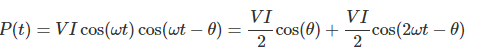
After applying the trig identity to the original expression for P(t), we see that AC power is the sum of two components. One of these is a constant, and the other is a sinusoid oscillating at 2ω. Both components have an amplitude of (V×I)/2.
The first component is the DC offset of the power waveform. The DC offset of a sinusoid is also the average value, and thus it’s not surprising that the first term is called the average power. As you can see, the average power is determined not only by voltage and current amplitudes but also by the cosine of the phase difference between voltage and current.
It’s important to recognize the relationship between this component of P(t) and what we have already learned about AC power:

As you may have already realized, average power is another name for active power. In other words, the average value of the sinusoidal power waveform conveys the amount of power actually dissipated by resistive components in the load circuit.
The second component of the P(t) expression accounts for the temporal fluctuations in power. In the context of real-life AC systems, the exact mathematical value of power at a given moment is not very important. Suppliers and consumers of electrical energy need to know how much energy is used over the course of an hour, or a day, or a month—the fact that the mathematical representation of AC power has short-term variations extending above and below an average value does not directly affect the long-term behavior of the power system.
However, this does not mean that the sinusoidal component itself is unimportant. The sinusoidal portion of P(t) gives us essential information about the nature of the load: As we learned in the previous chapter, if a waveform representing instantaneous power extends below the horizontal axis, the system requires reactive power. Furthermore, the amount of time that P(t) spends below the horizontal axis indicates the extent to which the system’s power factor deviates from the theoretically ideal value.
We’ve covered some important details related to the time-domain expression for AC power. We’ll continue this discussion in the next page as we incorporate P(t) into our understanding of RMS values and power factor.